
TL;DR: I’m going to show you how to take a fairly large dataset – in this case the galactic stars – and make some nice visualizations with a JavaScript library called D3. They look great.
Did you see the recent news from the ESA Gaia mission? It will eventually give the precise position and motion of one billion stars in our Galaxy (which is actually “only” one percent of the stellar population!). An initial release of data happened on 13th September 2016 and included the position, motion and distance of two million stars.
I wanted to take this data and play around with it and I like to play around with data with the help of D3. This is a web based visualisation tool, which unfortunately is restricted by the capabilities of today’s browsers. This means I’ve had to reduce the data points, however, I suspect we can still get some nice results.
I’ve downloaded some CSVs from Gaia’s archive website (http://cdn.gea.esac.esa.int/Gaia/), see the download page and select the tgas folder. I used some python code to select a subset of data points from the CSV’s and combine them into a single CSV, here’s that code:
import csv

filenames = [
	"TgasSource_000-000-000.csv",
	"TgasSource_000-000-001.csv",
	"TgasSource_000-000-002.csv",
	"TgasSource_000-000-003.csv",
	"TgasSource_000-000-004.csv",
	"TgasSource_000-000-005.csv",
	"TgasSource_000-000-006.csv",
	"TgasSource_000-000-007.csv",
	"TgasSource_000-000-008.csv",
	"TgasSource_000-000-009.csv",
	"TgasSource_000-000-010.csv",
	"TgasSource_000-000-011.csv",
	"TgasSource_000-000-012.csv",
	"TgasSource_000-000-013.csv",
	"TgasSource_000-000-014.csv",
	"TgasSource_000-000-015.csv"
]
with open("stars.csv", "w") as csvfileout:

	datawriter = csv.writer(csvfileout)
	getfirstrow = True

	count = 0
	for csvfilename in filenames :
		print( csvfilename )

		with open(csvfilename, "r") as csvfile:

			datareader = csv.reader(csvfile)

			skiprow = True
			for row in datareader:

				if getfirstrow :
					datawriter.writerow(row)
					getfirstrow = False

				if not skiprow :
					if count % 500 == 0:  # Change 500 to produce more or less data
						datawriter.writerow(row)

				skiprow = False
				count +=
All this does is open each CSV file, then select every 500th star (csv row). If we change the value 500 we can adjust the amount of data we obtain. This works because in the CSVs nearby stars are grouped together (and there’s a lot of them) so we get a fairly even selection of stars across the sky (this is likely just a consequence of how Gaia operates as it collects the star data), however there are “holes” where they shouldn’t be. One side note: whenever I start a D3 visualization I start with a drastically reduced dataset – I literally started with just 20 stars for this project, it makes debugging much simpler.
If you would prefer not to use python, then you can use this file with about 2000 stars in: https://bitbucket.org/akademy/gaiavis/src/26ddefef6dfb9adc0f50091bb836fbb06bace9cc/csvs/stars_skip_1000.csv. If you do publish anything remember to credit ESA and the Gaia groups:
This work has made use of data from the European Space Agency (ESA) mission Gaia (http://www.cosmos.esa.int/gaia), processed by the Gaia Data Processing and Analysis Consortium (DPAC, http://www.cosmos.esa.int/web/gaia/dpac/consortium). Funding for the DPAC has been provided by national institutions, in particular the institutions participating in the Gaia Multilateral Agreement.
Now we have some data let’s create something with it. First, you’ll need a place to put your D3 vis, so we’ll create a html file and with JavaScript create an SVG element with a width and height. We’ll need to include the D3 library too. Thus:
<html><body>
  <script src="https://d3js.org/d3.v4.min.js"></script>
  <script>
     var width = 1080, height = 520;
     var svg = d3.select("body")
                    .append("svg")
                    .attr("width",width)
                    .attr("height",height);
  </script>
</body></html>
Now we need to load the data and D3 makes this easy, we just need to request the file, and select the data we need from it.
d3.csv( "stars.csv", function(row) {
     // select data
     return {ra:row.ra *1, dec:row.dec*1};

}, function( data ) {
     // work with data
})
The filename here is “stars.csv”. The first function gets the two fields called “ra” and “dec” for each star (one csv row per star) and adds them to a small array. RA and Dec stand for Right Ascension and Declination respectively, this is just how we define a stars position and it’s literally how “right” it is (as opposed to “left”) from a defined start position and how high or low it appears from the Earth’s equator, (see Wiki’s Equatorial Coordinate System if you are interested). The “*1” after each value forces JavaScript to change the value into proper number. The second function receives all the data we have collected and we’ll need the “guts” of the code to go here.
This next bit might seem a little tricky but it’s just converting one number to another. We have lot’s of position data from loads of stars and we need to draw them inside our SVG. We do this by changing (called mapping or scaling) values from one to another. The RA and Dec numbers have defined maximum and minimum values (which we call their domain). For RA it’s 0 to 360, and for Dec it’s -90 to +90. In our SVG we will connect RA to the width and connect Dec to the height (we call this the range). We defined width and height variables at the beginning. In D3 we scale from one to the other like this:
var xScale = d3.scaleLinear()
         .domain([0,360])
         .range([0,width]);

var yScale = d3.scaleLinear()
         .domain([90,-90])
         .range([0,height]);
xScale will give the x position inside the SVG and yScale will give the y position inside the SVG.
Now we have to draw some stars, we’ll represent them as circles. To do this in D3 we attempt to select our circles and then draw them when it doesn’t find them – this sounds like the wrong way around but is a very powerful D3 way to manipulate elements based on a dataset. The code looks like this:
svg.selectAll("circle")
	.data(data)
	.enter()
	.append("circle")
	.attr("cx",function(d) { return xScale(d.ra); })
	.attr("cy",function(d) { return yScale(d.dec); })
	.attr("r", 1 )
First we (try) to select all circles but we haven’t created them yet, so we attach our data to this empty selection. We then call the function “enter()” which in our case means for each of the stars in our data which don’t have circles already (currently all of them) do this stuff that follows this function (think of “enter” in the same way as an actor enters the stage). So we append a circle. Then we add some attributes to it: SVG circles are defined by an x and y position (called cx and cy) and a radius (called r). The function in the cx attribute gets called with the piece of data (the CSV row, aka star) we are currently handling, here called d (as is standard for D3) and we select the ra value, we pass that value into our x scaler to find out where it need to be positioned. This is repeated for cy but this time using the dec and y scaler. The radius is always set to 1.
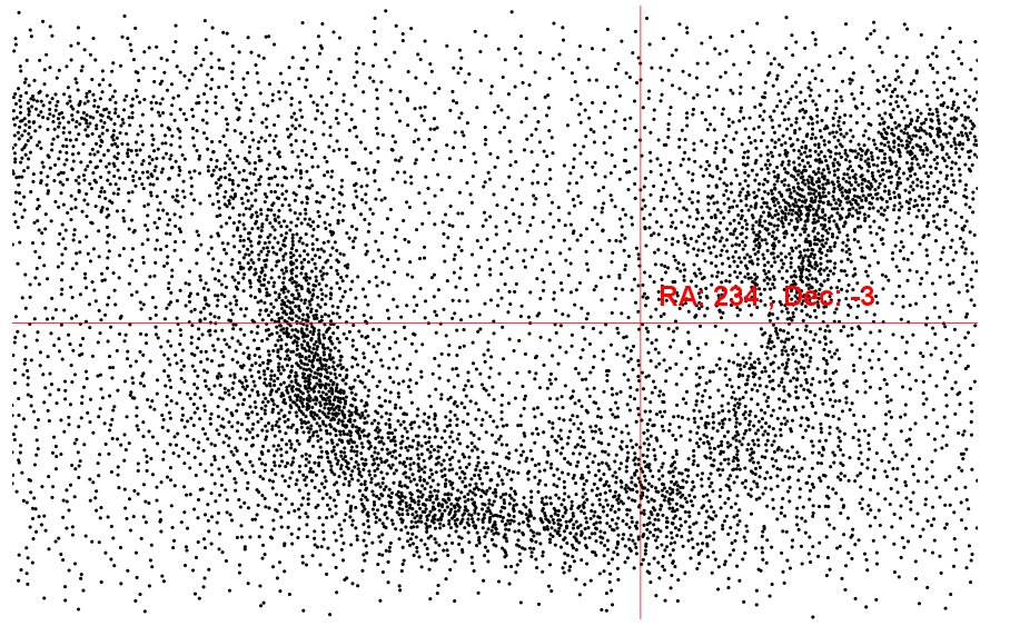
Great so, you should now be seeing something kinda awesome! Even with this few points you should be able to see a “path” of stars making what appears to be an arc across the SVG – this is the Milky Way, and it’s that funny shape as a consequence of the coordinate system. Isn’t it pretty!
We can make it prettier.
And in the next part we shall (We’ll make it more star like with the help of the flux measurement, play around with the positioning and make it more interactive ). See the next part here: Gaia star data with D3 – part 2 – prettier, faster
Check out the complete HTML file here https://bitbucket.org/akademy/gaiavis/src/26ddefef6dfb9adc0f50091bb836fbb06bace9cc/stars_basic.html
One Reply to “Gaia star data with D3 – part 1”